Graphing the belief in Allah

The blog-post by charles about using Bayes theorem and evidence from evolution to evaluate the probability of believing in God, which I also re-blogged, was interesting. As a scientist, what captivated me the most about the post was to “discover” some general trends between the prior and posterior at various values of likelihood.

I’m sure people may have done this sort of calculation before but I wanted to do it for my own personal understanding and for (yet) another blog entry.

In the true spirit of algebra (and following the reasoning of charles), I am replacing God with Allah and evolution with simply evidence. Here, evidence can be treated as any theory and/or observation that may be used as an argument, by the Muslims, to prove the existence of Allah. So, in this case, Bayes theorem can be stated as follows:

With the above equation in mind, I thought about checking how varying levels of likelihood affect the posterior. I, therefore, decided to plot a posterior vs. prior graph with varying levels of likelihood. The denominator of the right hand side of the above-stated equation i.e., P(Evidence), which also known as the normalizing constant, is often the most difficult to estimate. 

However, just to replicate the results of charles, I’ve decided to keep the analysis simple. The denominator can be re-written as:

Even though I am a scientist by training, I’ve decided to put on a philosopher’s hat for this exercise and assumed that the probability for any theory and/or observation that can be considered as evidence, given Allah does not exist, is 0.5. This is P(Evidence|NoAllah). 

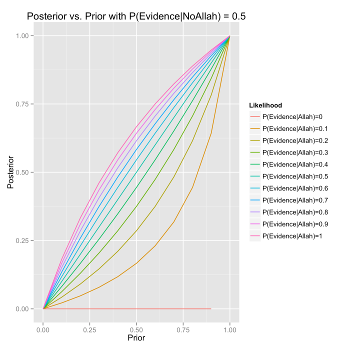
With these settings and assumptions, I produced the following graph:

Few interesting conclusions can be drawn from the graph:

1: Increasing the value of prior causes increase in the posterior.

2: The posterior always remains less than the prior when the likelihood is less than 0.5. At likelihood of 0.5, posterior and prior have same value. The posterior always becomes more than prior at likelihood of > 0.5. (Thanks to charles for pointing out this fact).

3: The higher the likelihood, the higher the posterior.

4: If the probability for evidence is 0, provided Allah exists, then no matter how strong the belief in Allah maybe, the posterior ends up being 0.

5: When the prior is 1 and likelihood is 0, the posterior cannot be calculated (as seen by incomplete red line on the graph). This is because P(Evidence) becomes 0 and dividing by 0 is undefined.

6: Prior value of 0 gives posterior value of 0 at all levels of likelihood. Likewise, prior value of 1 gives posterior value of 1 at all levels of likelihood.

This, I believe, nicely complements the blog-post by charles and summarizes some key relations between various variables in Bayes theorem.

And, finally, for the more curious and technical-minded, following is the code in R programming language I used to produce the graph in this blog-post:

require(ggplot2)

bayes_theorem <- function(pg,peg,pegn){
	pgn = 1 - pg
	pge = (peg*pg)/((peg*pg)+(pegn*pgn))
	return (pge)
}

graph_data <- function(prior){
	allvals <- c()
	for (x in prior){
		allvals <- append(allvals,bayes_theorem(prior,x,0.5))
	}
	df <- data.frame(x=rep(prior,length(prior)),val=allvals,variable=rep(paste0("P(Evidence|Allah)=", prior), each=length(prior)))
	names(df) <- c("x","val","Likelihood")
	g1 <- ggplot(data=df, aes(x=x,y=val)) + geom_line(aes(colour=Likelihood))
	g1 <- g1 + ylab("Posterior") + xlab("Prior") + ggtitle("Posterior vs. Prior with P(Evidence|NoAllah) = 0.5")
	ggsave(g1,file="prior_posterior.png")
	return(g1)
}

prior <- seq(0,1,by=0.1)
graph_data(prior)